What makes a program “better”?
There are multiple ways of measuring if a program is “better” than an other, assuming they perform similar functions:
- Correctness: a program not producing the correct output is worst than a program that is always correct,
- Security: a program leaking personal information or infesting your computer will always be worst than one that does not,
- Memory: the less a program requires memory to be installed and to run efficiently, the better.
- Time: the faster the program produces the output, the better.
- Other measures: ergonomics, cost, compatibility with operating systems, licence, network efficiency, may also come into play to decide which program is “best”.
Some criteria may be subjective (usability, for example), but some can be approach objectively: in a first approximation, memory (also called “space”) and time are the two preferred measures.
Orders of magnitude in growth rates
Principles
When measuring space or time, it is important to take the size of the input into account: that a word-processing software can open a document containing 1 word in 0.0001 second is no good if it takes hours to open a 10 pages document.
Hence, algorithms and programs are classified according to their growth rates, how “fast” their run time or space requirements grow when the input size grows. This growth rate is classified according to “orders”, using the Big O notation, whose definition follows:
Using to denote the absolute value, we write:
if there exists positive numbers and such that
for all .
Stated differently, the size of ‘s output (which we will use to represent the time or space needed by to carry out its computation) can be bounded by the size of ‘s output,
- up to a multiplicative factor () that does not depend of (it is fixed once and for all),
- for inputs that are “large enough” (that is, greater than , which again does not depend on , it is fixed once and for all).
Common orders of magnitude
Using for “a constant”, for the size of the input and for logarithm in base , we have the following common orders of magnitude:
- constant (),
- logarithmic (),
- linear (),
- linearithmic (),
- polynomial (), which includes
- quadratic (),
- cubic (),
- exponential (),
- factorial ().
Simplifications
In typical usage the notation is asymptotical (we are interested in very large values), which means that only the contribution of the terms that grow “most quickly” is relevant. Hence, we can use the following rules:
- If is a sum of several terms, if there is one with largest growth rate, it can be kept, and all others omitted.
- If is a product of several factors, any constants (factors in the product that do not depend on ) can be omitted.
There are additionally some very useful properties of the big O notation:
- Reflexivity: ,
- Transitivity: and implies ,
- Constant factor: and implies ,
- Sum rule: and implies ,
- Product rule: and implies ,
- Composition rule: and implies .
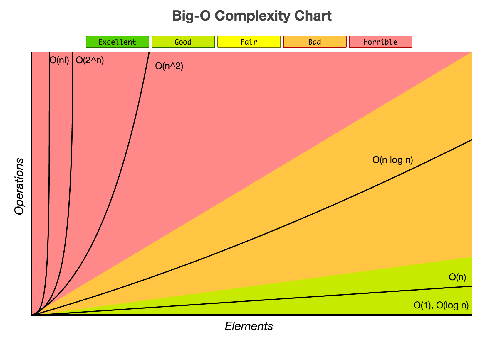
Have a look at the Big-O complexity chart:
Experimentation
How fast a function grows can make a very significant difference, as
exemplified in this code available to
download. In it, we “experiment”
to see how fast factorial, exponential, cubic, quadratic, linearithmic,
linear and logarithmic functions can produce an integer that is larger
than int.MaxValue, whose value is .
For example, the test for exponential growth is as follows:
    int inputexp = 0;
    int outputexp;
    try
    {
      while (true)
      {
        inputexp++;
        checked
        {
          outputexp = (int)Math.Pow(2, inputexp);
        }
      }
    }
    catch (System.OverflowException)
    {
      Console.WriteLine(
        "Exponential: an overflow exception was thrown once input reached "
          + inputexp
          + "."
      );
      // Exponential: an overflow exception was thrown once input reached 31.
      // 2^31 = 2,147,483,648
}C#‘s default Math.Pow method returns a double (because, as you will
see, producing something an int cannot hold goes very fast), so we
cast it back to an int, in a checked environment so that C# will
raise an exception if an overflow occurs. Our while(true) loop will
terminate, since we are bound to produce a value overflowing, and then
we simply display the value our input reached: in this case, it was
enough to “feed” the value to the exponential function to make it
go over int.MaxValue.
Download the project to see how
fast other magnitude produce a value exceeding int’s capacity, and do
not hesitate to edit this code to have all input values starting at 0 to
“feel” the difference it makes in terms of time!
The Example of Integers
Abstraction and Representation
To measure the time and space consumption of programs, we make some simplifying assumptions:
- Hardware is discarded: we compare programs assuming they run on the same platform, and do not consider if a program would be “better” on parallel hardware.
- Constants are discarded: if a program is twice as slow as another one, we still consider them to be in the same order of magnitude1.
- Representations are in general discarded, as programs are assumed to
use the same: for example, if the implementation of the
intdatatype is “reasonable” and the same for all programs, then we can discard it.
How “reasonable” is defined is tricky, and we discuss it in the next section.
How integers are represented
Compare the following three ways of representing integers:
| Name | Base | Examples | Bits to represent |
|---|---|---|---|
| Unary (Tallies) | 1 | III, IIIIIII, IIIIIIII, … | |
| Binary | 2 | 01011, 10011101, 101101010, … | |
| Decimal | 10 | 123, 930, 120,439, … |
It takes roughly digits to represent the number in base , except if .
And indeed we can confirm that for , we have
by changing the base of the logarithm.
Why it (almost) does not matter
Now, imagine that we have a program manipulating integers in base , and we want to convert them in base . We will ignore how much time is required to perform this conversion, and simply focus on the memory gain or loss.
| Base | Size of |
|---|---|
| Base | |
| Base |
Hence, converting a number in base into a number in base results in a number that uses more (or less!) space. Notice, and this is very important, that is expression does not depend on , but only on and , hence the “constant factor” property of the big O notation tells us that we do not care about such a change.
For example, going from base to base means that and , hence we need times more space to store and manipulate the integers. This corresponds intuitively to 32 bits being able to store at most a 10-digit number (2,147,483,647).
If our program in base uses memory of order , it means that a program performing the same task, with the same algorithm, but using integers in base , would have its memory usage bounded by . By adapting the constant factor principle of the big O notation, we can see that this is a negligible factor that can be omitted.
However, if the base is 1, then the new program will use : if is greater than linear, this will make a difference2. Of course, unary representation is not reasonable, so we will always assume that our representations are related by some constant, making the function order of magnitude insensible to such details.
You can have a look at the complexity of various arithmetic functions and see that the representation is not even discussed, as those results are insensible to them, provided they are “reasonable”.
Types of Bounds
Foreword
When considering order of magnitude, we are always asymptotic, i.e., we consider that the input will grow for ever. The Big-O notation above furthermore corresponds to the worst case, but two other cases are sometimes considered:
- Best case,
- Average case.
The first type of study requires to understand the algorithm very well, to understand what type of input can be easily processed. The second case requires to consider all possible inputs, and to know the distribution of cases.
The reason why worst case is generally preferred is because:
- Worst case gives an upper bound that is in practise useful,
- Best case is considered unreliable as it can easily be tweaked, and may not be representative of the algorithm’s resource consumption in general,
- Average case is difficult to compute, and not necessarily useful, as worst and average complexity are often the same.
Examples
Linear search algorithm
The linear search algorithm looks for a particular value in an array by inspecting the values one after the other:
    int[] arrayExample =
    {
      1,
      8,
      -12,
      9,
      10,
      1,
      30,
      1,
      32,
      3,
    };

    bool foundTarget = false;
    int target = 8;

    for (int i = 0; i < arrayExample.Length; i++)
    {
      if (arrayExample[i] == target)
        foundTarget = true;
    }
    Console.WriteLine(
      target + " is in the array: " + foundTarget + "."
);How many “steps” of computation are needed? The operations inside the loop themselves can be discarded, since they are a finite number, but what matter is how many time those operations are performed, that is, how many time the loop iterate.
Considering that the array is of size , we have:
- The best case is if the target is the very first value, in this case, the time complexity is .
- The worst case is if the target is the very last value (or is not in the array), in this case the time complexity is .
- The average case is .
This algorithm can be slightly tuned, to exit as soon as the target value is found:
    bool foundYet = false;
    target = 30;
    int index = 0;

    do
    {
      if (arrayExample[index] == target)
        foundYet = true;
      index++;
    } while (index < arrayExample.Length && !foundYet);
    Console.WriteLine(
      target
        + " is in the array: "
        + foundYet
        + "\nNumber of elements inspected: "
        + (index)
        + "."
);Similarly, considering that the array is of size , and counting how many time the loop iterate, we have:
- The best case is if the target is the very first value, in this case, the time complexity is , for a constant value.
- The worst case is if the target is the very last value (or is not in the array), in this case the time complexity is .
- The average case is .
Note that the space usage of both algorithms are , as they require only one variable if we do not copy the array. Note, also, that both algorithms have the same worst case and average case complexity, which are the cases we are actually interested in.
Binary search algorithm
The binary search algorithm looks for a particular value in a sorted array by leveraging this additional information: it “jumps” in the middle of the array, and if the value is found, it terminates, if the value is less than the target value, it keep looking in the right half of the array, and it keeps looking in the left half of the array otherwise.
What is the (worst case) time complexity of such an algorithm? It halves the array at every step, and we know that if the array is of size , then it will terminate (either because the value was found, or because it was not in the array). That means that, if the array is of size , in the worst case,
- after step, we have an array of size left to explore,
- after steps, we have an array of size left to explore,
- after steps, we have an array of size left to explore,
- … after steps, we have an array of size left to explore.
Hence, we need to determine what is a such that
since we terminate when the array is of size . It is easy to see that if , then this will be true, hence , as .
Matrix Multiplication
Consider the “schoolbook algorithm for multiplication”:
  static int[,] MatrixMultiplication(
    int[,] matrix1,
    int[,] matrix2
  )
  {
    int row1 = matrix1.GetLength(0);
    int column1 = matrix1.GetLength(1);
    int row2 = matrix2.GetLength(0);
    int column2 = matrix2.GetLength(1);

    if (column1 != row2)
    {
      throw new ArgumentException(
        "Those matrixes cannot be multiplied!!"
      );
    }
    else
    {
      int temp = 0;
      int[,] matrixproduct = new int[row1, column2];

      for (int i = 0; i < row1; i++)
      {
        for (int j = 0; j < column2; j++)
        {
          temp = 0;
          for (int k = 0; k < column1; k++)
          {
            temp += matrix1[i, k] * matrix2[k, j];
          }
          matrixproduct[i, j] = temp;
        }
      }

      return matrixproduct;
    }
}We can see that
- The first loop iterates
row1times, - The second loop iterates
column2times, - The third loop iterates
column1times,
If we multiply square matrices, then row1, colmun2 and column1 are
all equal to the same value, , that we take as input of the problem:
then we can see by the product rule above that this algorithm requires
time to complete.